Who the Devil is Maxwell?

Siraj Sabihuddin

A scientist, engineer and maker trying to understand physics.

Maxwell? Who is he? Why should we even care who he is? And ohhh … god! What is the insanity behind his equations?! … these my friends are the questions that run chills down the spines of us normal folks. We are like fish out of water, thrashing about in an insane desperate struggle to comprehend the great questions of the universe. Well, lets try diving back into the ocean … and gaze upon the incredible deliciousness of physics at work.

Disclaimer: This article was originally written on May 29, 2012 and is a republished from my old blog which was hacked. Sigh. Yes.

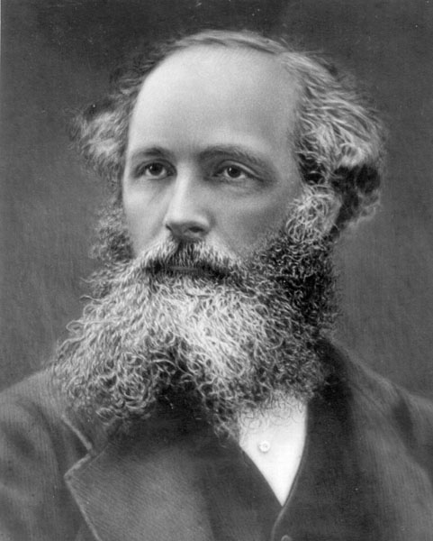
There are a huge number of representations for Maxwell’s equations. The picture below shows a portrait of Maxwell who brought together the contributions of various other scientists into what is now known as Maxwell’s equations.

One of these representations is presented below. A key difficulty in understanding these equations on the net, is that many different unit systems exist. The set of equations below follows S.I. units – which at the moment is the preferred representation. A further difficulty is that, some representations do not correctly use the variables: D, P, E, H, M, B –  a fair amount of confusion exists on how these variables should be used. I have tried to choose the most accurate representation that I can find. Don’t worry! I’ll get to what it all means!

Gauss’ Electric Field Law

{\phi}_{\small{E}} = \oint_{S}{\vec{D} \cdot d\vec{A}} = Q \tag{1}

Gauss’ Magnetic Field Law

{\phi}_{\small{M}} = \oint_{S}{\vec{B} \cdot d\vec{A}} = 0 \tag{2}

Faraday Maxwell Law

\varepsilon_{ind} = - \oint_{C}{\vec{E} \cdot d\vec{l}} = - \frac{\partial {\phi}_{\small{M}}}{\partial t} \tag{3}

Ampere Maxwell Law

\mathcal{F_{ind}} = \oint_{C}{\vec{H} \cdot d\vec{l}} = \frac{\partial {\phi}_{\small{E}}}{\partial t} + I \tag{4}

The above representation is the integral form of Maxwell’s equations – these equations look slightly different from the forms you may have seen, however, they’re not – I promise! Ok .. wait … I’d better not … ummm … so, I’ve redefined them so that they are a bit more symmetric and both versions of Gauss’s law use the material dependant electric and magnetic fields. I also fixed Faraday and Ampere-Maxwell’s lawas so that both versions use the material independant electric and magnetic fields …. anyways! … moving on … These equations can also be written in differential form as shown below. The two forms are mathematically identical.  The differential form can be derived from the integral form by using the divergence theorem.

Gauss’ Electric Field Law

\nabla \cdot \vec{D} = \rho \tag{1A}

Gauss’ Magnetic Field Law

\nabla \cdot \vec{B} = 0 \tag{2A}

Faraday Maxwell Law

\nabla \times \vec{E} = - \frac{\partial \vec{B}}{\partial t} \tag{3A}

Ampere Maxwell Law

\nabla \times \vec{H} = \frac{\partial \vec{D}}{\partial t} + \vec{J} \tag{4A}

Occasionally some people also add one additional equation to this rather heady mix of mathematics:   the Lorentz Force (sometimes also known as the Laplace force). I have sneaking suspicion that this force can actually be derived from Maxwell’s four equations … alas, I’m not sure – at some point I’ll work up the nerve to actually give it a go! 

Lorentz Force Law

\vec{F} = \vec{F}_{\;\small{E}} + \vec{F}_{\;\small{M}} =  Q \cdot (\vec{E} + \vec{v} \times \vec{B}) = Q \; \vec{E} + \vec{J} \times \vec{B} \tag{5}

Well then!  There you have it!  Now where to go from here?  Well, let’s see whether my imperfect (and very much incomplete) knowledge can break all this down in to something that makes sense.  You’re probably asking yourself, “What do all those pesky variables mean?” …  Well, in order to understand these equations there’s a whole lot of the basics to go through.   Lets get on with it! … UPDATE: I’ve recently discovered that a wonderful and detailed discussion of theory was presented by Richard Feynman in his lecture series [1] in the 1960’s. I encourage readers to look at this series for more explanations on the topics I’m discussing.

1. Electric Charge (Q, q) and Charge Density (ρ)

Let’s start at the very beginning with our little friend, the humble little Q in our Lorentz force equation (equation 5). The value Q is a variable representing the total electric charge, and is measured in a unit called the Coulomb denoted as [C].

Total Electric Charge 

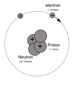
Q = \sum_{i=0}^{n}{q_i} \tag{6}

Every atom is composed of a heavy and dense nucleus containing  protons (+ charge) and neutrons (no charge).  Around this nucleus orbit electrons (– charge). In-fact, it turns out that protons and electrons have equal and opposite charge. That is, specifically -1.6 x 10^-19 [C] for an electron and 1.6 x 10^-19 [C] for a proton.   Sometimes, we can also denote charge as, q. For this article I will use this small letter to denote a point charge (equation 6) with unit [C].

We can also represent charge in another form: as the charge density. This assumes that a space is a continuous distribution of charge as opposed to one with discrete point charges. The charge density, is thus, defined per unit volume and is denoted ρ and measured in units [C/m³] as shown in the equations below. The value, V represents the volume of the electrically charged object.

Total Charge

Q = \int_{V}{\rho\;dV} \tag{6A}

Charge Density

\rho = Q/V \tag{7}

So electrons and protons are the charge carriers.  Protons are, typically and to present day, very difficult to remove from an atom.  However, with the addition of some energy it’s possible to knock or drag electrons off of an atom.  How easy or difficult it is to knock an electron off an atom has a lot to do with it’s quantum properties and is a subject best left for another day.

Figure 1 is a representation of an atom as described earlier. Modern quantum theory models an atom quite differently – electrons exist as clouds and occupy shells. But as I mentioned before … that’s a topic for another day.

2. Coulomb’s Law and Electrostatic Force (F_E) 

Now, the one property we are all familiar with is the idea that opposite charges attract and like charges repel. We can formalize this idea in terms of (electrostatic) forces.  This formalized idea is what we call Coulomb’s Law and is represented below:

Coulomb’s Law

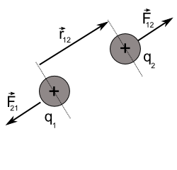
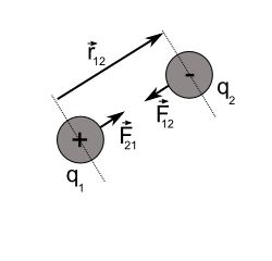
{\vec{F\;}}_{12} = k \; \frac{q_{1} \; q_{2}}{{||\vec{r\:\;}_{12}||}^2} \; \hat{r}_{12} \tag{8}

As seen in figure 2a and figure 2b, q₁ and q₂ represent two point charges.  These point charges are sometimes known as electric monopoles. F₁₂ is the force in, Newtons [N], exerted on point charge 2 by charge 1. It is directed away from 1 (for like charges) and towards 1 (for un-like charges).  Likwise, F₂₁ is the force on charge 2 as a result of charge 1. The value r₁₂ is a representation of the vector distance between charges 1 and 2 directed from 1 to 2.  The magnitude of this vector, the distance, is measured in meters [m]. Notice also that [N]=[Kg m/s²].

But hold on a sec!  What’s this mysterious letter, k, sitting right there at the front of Coulomb’s law? Well, that my friends, is a proportionality constant,  a.k.a. Coulomb’s constant.  It’s a representation of the medium in which the charges are immersed.  It’s defined below.

Coulomb’s Constant

k = \frac{1}{4 \; \pi \; {\epsilon}} \tag{9}

ϵ is defined as the permittivity …. Whooa!  Permittivity?! Okay … we’ll talk about this in a moment! But before that, if there are more than two point charges (or electric monopoles) in a given system the force on any given charge would be the vector sum of the individual forces exerted by all the other charges on that particular charge (denoted with subscript i).  This sum is also known as the superposition principle. So we could rewrite the force above as follows:

Coulomb’s Law

\vec{F}_{\;\small{E}} = \sum_{\substack{i,j=0 \\ i \neq j}}^{n}{k \; \frac{q_{i} \; q_{j}}{{||\vec{r\:\;}_{i \; j}||}^2} \; \hat{r}_{i \; j}} \tag{8A}

Notice that this force is always relative to some existing charge in space. The force doesn’t exist on uncharged particles – this is not completely true (we can induce what are called electric dipoles). Now we’re ready to move on! Oh wait! One more thing. We can represent this force in one other way using something called an electric field – more on this further down.

3. Permittivity & Electric Susceptibility

The permittivity is a measure of how well a particular medium or material permits the transmission of our electrostatic force.  It’s defined in the equation below:

\epsilon = {\epsilon}_{r} \cdot {\epsilon}_{0} = (1+{\chi}_{\small{E}}) \cdot {\epsilon}_{0} \tag{10} 

ϵ_r is the relative permittivity (a.k.a. dielectric constant) and is specifically dependent on the medium or material, while ϵ₀ is the permittivity of free space  and is independent of the medium.  In a vacuum, ϵ_r = 1, so ϵ=ϵ₀​≈8.85 x 10⁻¹² [C²s²kg⁻¹m⁻³] … sigh … we’ll discuss the units a bit later on. The permittivity of a material is a result of the intrinsic atomic and molecular properties of the material.

χ_e is known as the electric susceptibility and is a dimensionless quantity. Likewise, the relative permittivity must then also be dimensionless.  Sometimes it’s more useful to think of susceptibility rather than relative permittivity.  The susceptibility pertains to how willingly a material changes (or polarizes) in response to electrostatic influences.  To talk more about this, we really need to introduce the concept of  electric fields  … so lets move on for now.

4. Electric Fields  

So Coulomb’s law models electrostatic forces.  In the real world, force is the only thing that can be truly measured.  Brilliant!!  ….. But, wait a second …. there’s more.  You see, electrostatic force on a given charge is dependent on another charged particle.  Sometimes a more general representation is needed – enter the electric field.  This electric field, E is a vector field and because it is no longer dependent on another particle can be defined at all points in space. 

Let’s suppose we start with a single charge in space, call it Q.  If we now bring in a small positive test charge, q, at some radius r the test charge now experiences some force, F_E. Let’s assume that for now only these two charges exist … then we can rewrite Coulomb’s law as follows.

Coulomb’s Law

{\vec{F}_{\;\small{E}}} = k \cdot \frac{Q \cdot q}{{||\vec{r}||}^2} \cdot \hat{r} \tag{8B}

Taking this, we can create a representation that is independent of the small positive test charge.  This independent representation is called the electric field and is defined mathematically below.

Electric Field

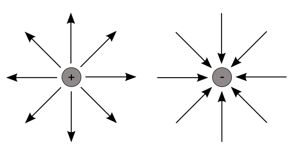
{\vec{E}} = \frac{{\vec{F}_{\small{E}}}}{q} \tag{11}

The electric field is the force per unit charge and so is assigned units [N/C]. Going back to the idea of permittivity, we can see that like the electrostatic force, the electric field is also dependent on the material through which it propagates. An electric field generated by a positively charged particle will repel a positive test charge and likewise, attract a negative test charge. Thus, by convention, electric fields point away from positive charge and towards negative charge. Figure 3 shows electric fields (at discrete points in space) for positive and negative point charges. 

As we can see in figure 4, more complex field configurations are also possible.  The figure shows a 2D field, generated in Matlab, around a set of charged particles, but obviously most day to day systems are three dimensional and so you can imagine the field extending out in all directions including into and out of the page.

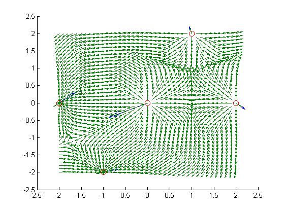
Furthermore, the figure shows these fields as discrete quantities with constant field strength over the entire space. In reality these fields are continuous and exist every where in space, dropping off as the square of the radial distance from the source charge (as indicated by our force, F_E in equation 8).  A point worth noting, is that if a group of charges (as shown in the figure) exist in some geometry and we are very distant from this group, then they start to behave much like a point charge.  

6. Free & Bound Charge (Displacement D & Polarization P)

If we look at any system containing an electric field, for instance one consisting of an object and air, then we see that there are two ways in which charge exists. Charges may be free to move around or they may be bound to a particular region in space.

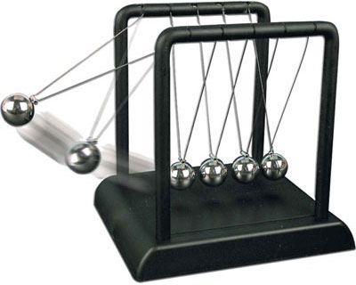
As we saw earlier, a positive/negative test charge in space undergoes a force, F_E within an electric field E. Obviously, if this charge is not attached to something, then it will move and hence it is considered a free charge. Conductors are an example of materials that have many free charges associated with them – outer valence electrons in conductor atoms are loosely bound and can break free very easily under the influence of an electric field. In a sense, the conductivity of a conductor can be linked to how easy or difficult it is to break that initial bond for these electrons. The electrons propagate through the conductor by knocking neighbouring electrons much like a Newton’s Cradle (figure 6). Beware folks! I’m being very liberal by describing a conductor and free charge in this way.  There are quantum mechanical effects at work that I just don’t understand well enough to go beyond this explanation. Even in conductors there’s a limit to how much these electrons move. One term often bandied about is electron drift velocity – which in conductors despite the speed of propagation of “electricity” tends to be quite low. 

A bound charge is one whose range of motion is quite limited and cannot break free from its atom easily. Materials that exhibit strong binding of this sort are often termed as insulators. It is extremely difficult to move charges into or out of this insulating material, however, a field applied to this insulator can induce an electric dipole in the material. This phenomenon is known as electrostatic induction. Actually, inductive effects are also experienced by conductors. Every material has an electronegativity & electron affinity. The electronegativity indicates how strongly a material attracts electrons to it. The electron affinity is the energy released on capture of an electron by a neutral atom to form a negative ion. For insulators, rubbing a material with high electronegativity (or high affinity) with one with low electronegativity (or low affinity) causes an exchange of electrons and a net charge on an otherwise neutral object.

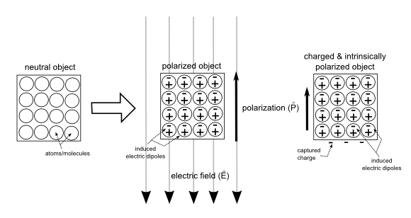
Because of free and bound charges, we can actually define a value called the electric displacement field, D. The next equation provides a mathematical definition. The units for D are [C/m²]. This field represents the sum total contribution of both free and bound charges resulting from the application of an external electric field, E. When this external field is applied to some material it undergoes a response via electrostatic induction and polarizes. The effect of this induction is an electric dipole and is indicated by the electric polarization, P of the material measured in [C/m²].

\vec{D} = \epsilon_0 \; \vec{E} + \vec{P} \tag{13}

Most objects in nature tend to have neutral charge. And so the intrinsic electric polarization is zero – though insulators may pick up charge with great difficult via rubbing, for instance. An insulator that picks up charge in this manner exhibits an intrinsic electric dipole induced by this extra charge (figure 6). Some materials may also have a molecular polarization resulting from the shape of their molecules.

If indeed there is no intrinsic polarization then the polarization is strictly a result of the external electric field and is linearly proportional to this external field (figure 6). This linearity shown in the equation below: 

Electric Polarization

\vec{P} = \epsilon_0 \; \chi_{\small{E}} \; \vec{E} \tag{13}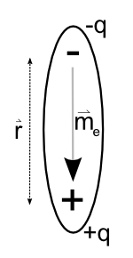

In insulators the polarization elongates molecules or atoms such that electrons spend more time, on average at one end of the atom. In conductors the situation is slightly different since the charges are not bound and can collect at one end of the material – I think this would mean that conductors exhibit stronger polarization. Its important to note that if electrons are flowing in and out of a conductor, for instance in a circuit, then the net electric field inside the conductor would be zero. 

Since we’ve been talking about electric dipoles and polarization, there’s another quantity worth mentioning, namely the electric dipole moment. Looking at figure 8, then we see that the dipole moment can be defined as follows:

Electric Dipole Moment

\vec{p} = q \; \vec{r} \tag{14}

Electric Dipole Torque

\vec{\tau}_{\small{E}} = \vec{p} \times \vec{E} \tag{15}

An external field applied to this dipole results in a torque, τ_E​. Furthermore, from this moment we can calculate the resultant polarization field as shown in the next equation. Notice that N is the number of charges in the system – this number is sometimes combined with the the electric moment as shown by the equivalence in the equation below.

Electric Polarization

\vec{P} = N \; \frac{\vec{p}}{V} \equiv \frac{1}{V} \cdot \vec{p} \tag{13A}

With that, we’re ready to tackle the concept of electric flux and then to the first of Maxwell’s equations: Gauss’ Electric Field Law! So lets get too it!

5. Electric Flux 

We saw that for point charges the electric field was distributed evenly, spherically around the the point charge. Suppose we took a small surface on some arbitrary spherical surface, S, centred at our point charge, Q (figure 5a).

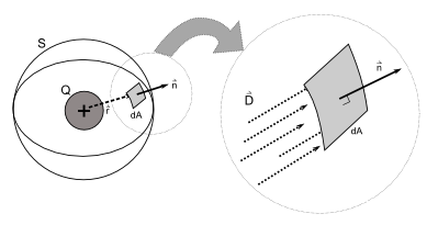
Further, lets take some tiny area, dA, on that sphere S. The electric field at that surface, at a radius, r, is given by E. Wait, not quite … a more correct representation would be D – this displacement field also takes into account the material through which the electric field is propagating. We see that a number of electric field lines emanate radially out from the charge, Q and pierce this surface. So we can define the quantity of electric field lines piercing the surface as D ⋅ dA. The total amount of field lines intersecting a surface is known as the electric flux, ϕ_E​ through that surface. In our case all our electric field lines are parallel to the normal vector, n of our tiny surface. But this may not always be true. In-fact we don’t need to choose a spherical surface S. We can choose a plane as shown in figure 5b. In this case the electric field may pierce the plane at different angles. Only the field lines parallel to the normal of that surface, n have any contribution to the total electric flux. And further more if we really look at the entire surface, S, rather than a small area, dA, the flux is just the sum of all the little dA elements. We can compute the flux as shown in the equation below.

Electric Flux through Surface

{\phi}_{\small{E}} = \int_{S}{\vec{D} \cdot \vec{n} \cdot dA} = \int_{S}{\vec{D} \cdot \vec{dA}} \tag{12}  

Notice that the equation contains a dot product D ⋅ n ⋅ dA to indicate that only the components of the electric field parallel to the normal vector of the surface at the given location are contributing to the total flux. Its clear that if the vectors D and n were perpendicular then the dot product would be zero. Normally, in text books, the multiplication n ⋅ dA is represented as dA for the sake of convenience. Since the dot product is a scalar value, we can also expect the electric flux, ϕ_E to be scalar. It also follows from our equation that the electric flux would be measured in units of [N m²/C]. 

At this point, I need to make it absolutely clear that the flux definition above is NOT how it is defined in most textbooks or on the web. The standard definition for flux (and as a consequence, Gauss’ Law) is ϕE​=∫_S​E⋅dA. The reason for my re-definition lies in the fact that the four Maxwell’s equations should be defined in a symmetric fashion. Gauss’ Magnetic Field Law is defined with the material dependent B field such that B = μ₀ ⋅ (H + M). So Gauss’ Electric Field Law should also be defined in a material dependent fashion with the D field such that D = ϵ₀​E+P.

7. Gauss’ Electric Field Law

As a reminder, I’ve re-iterated Gauss’ Electric Field Law in both integral and differential form in the equations below. Now! Lets try to bring everything we’ve looked at together and make beautiful music!

Gauss’ Electric Field Law 

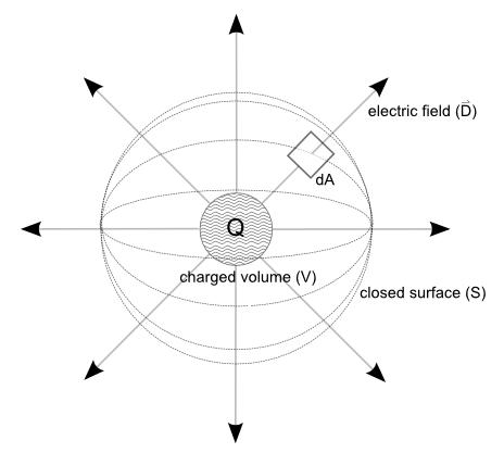
{\phi}_{\small{E}} = \oint_{S}{\vec{D} \cdot d\vec{A}} = Q \tag{1}

\nabla \cdot \vec{D} = \rho \tag{1B}

Hmmm … but how to explain this? Well, lets try to paint a picture … if we were to imagine a space containing charge, Q, then the flux going through some arbitrary closed surface, S around Q would be proportional to the volume of charge, V, enclosed by the surface. Confused? Me too!!!!  Maybe a picture will help? Here’s one.

Here’s a simpler version of Gauss’ Law. Don’t forget how the Q is defined in this equation, either.

Gauss’ Law

{\phi}_{\small{E}} = Q \tag{1}

Total Charge

Q = \sum_{i=0}^{n}{q_i} = \int_{V}{\rho\;dV} \tag{6}

With this equation, its possible to determine the electric field going through any surface of your choice. But, like any good puzzle, there’s a catch. 

The catch is that you have to choose the right surface for the right charge configuration. If you choose some arbitrarily complex surface then the problem becomes much much much more difficult to solve.  The key is to look at the symmetry of the problem and use that as a basis of surface selection.

If you look at the charge Q, it takes the shape of a sphere. So the emanating electric field, E will point out of the charge radially. If we now choose our closed surface, S, such that it is spherical, also and centered at the centre of Q then every intersecting field line will be perpendicular to the surface and hence our dot product, D ⋅ dA will become a simple scaler product. 

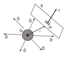
Now suppose we have another sort a charge distribution. Have a look at the next figure. In this case the charge is spread out over a plate as shown in the figure below. If we were to take our surface as a sphere, then the problem becomes quite hard … where as if we assume a pillbox (cube) surface things are much easier.

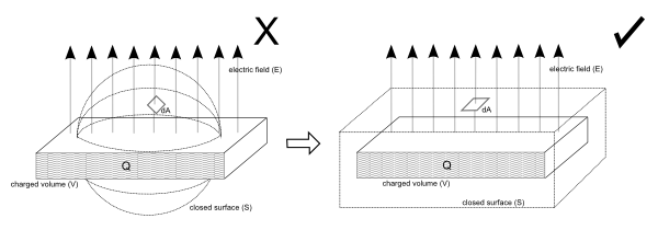
In this case (right image), the electric field pierces both the top and bottom surface of the pillbox, parallel to the surface normal. This makes it much easier to solve than the spherical surface on the left. For the spherical surface, the radial distance of the charge changes for every point on it. As well the angle at which the electric field interacts with the surface also changes. 

There you have it! The remaining three Maxwell equations require an introduction to magnetostatics. So let’s get on with it! Oh … one sec.  Before we get to magnetic fields we need to discuss the implications of bound and free charges a bit more and introduce the idea of current, resistance and emf. Lets do that first.

8. Electric Current (I, J)

Earlier, I talked about bound and free charge, that naturally leads to another concept: the electric current. Electric current is a way of representing moving charge, often in the form of electrons. This moving charge, because it is moving, must necessarily be free charge. …. wait wait, I take that back, if we think of bound charge – this charge also undergoes some very limited motion, so in some sense may also contribute to a very short duration current flow when the charge first moves into its induced position. 

Normally the current is represented as, I. This representation of current is used extensively in situations where wires are concerned – where we can assume that the current behaves as a one dimensional (line-like) quantity. We might think of current as an average quantity telling us roughly what is happening in a wire.  In reality, current is not a one dimensional quantity. A more general representation called the current density, J is sometimes used. Here’s a figure to give you a sense of what this all means. 

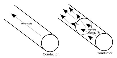
Current density, J, is a vector field. In-fact we can formally define both current and current density as shown in the next equation. An unfortunate historical choice has defined the current as flowing in a direction opposite to that of electrons. Really, it is the electrons that move and define current flow, but back in the day when people were busy discovering new things about electricity they had to decide a direction. There was a 50/50 chance of getting it right … alas it was the wrong choice, what can you do? … I mentioned electrons, but current can be a result of any moving charge – even at the macroscale … these macroscale objects are sometimes known as charge carriers. 

Current

I = \frac{Q}{t} = \frac{dQ}{dt} = \int_{S}{\vec{J} \cdot d{\vec{A}}} \tag{16}

Current Density

\vec{J} = \frac{I}{\vec{A}} \tag{17}

We define current, I as the current density flux through some cross-sectional surface, S, in a material. This current is usually measured in Amperes [A] = [C/s]. The current is the measure of the total amount of charge, Q that flows through a particular cross-sectional area, A in some amount of time, t. Likewise the current density, J, is defined as the amount of current per unit area (measured in units [A/m²]. The area being the cross-sectional area through which the current is passing. 

Mobile charges in a conductor (or insulator) move randomly in various directions. When an external magnetic field is applied, these electrons start to drift at what is known as: v_d, the electron (average) drift velocity. To give us a sense of what this means, we can compare this drift to the motion of air. Under the influence of an electric field this drift velocity is computed using the equation below:

Electron (average) Drift Velocity

\vec{v}_{d} = \frac{I}{N\;A\;Q} = u \; \vec{E} \tag{18} 

Note that the value, u is the electron mobility measured in [m2/V s], with [V] = [Nm/C] being the voltage. I’m not completely certain here, since I haven’t been able to find a definitive answer … but I believe that electron mobility is dependent on the properties of a material and should be available in a table somewhere. Its interesting to note that in a vacuum, electrons travel in a straight line at nearly the speed of light. However, inside a material, this velocity can be very low – in the order of millimeters per second [mm/s]. But how come electrical signals travel very fast through a conductor? A way of thinking about this is to look at the propagation of sound through air. The pressure wave passes through air much faster than the motion of any individual particle.  The same is true for current which propagates through a conductor very fast relative to the individual charge carriers. 

Since we’re already talking about current, lets briefly discuss a little bit more about free charge and conductors. Earlier I mentioned that conductors don’t really have an electric field inside them. That’s not completely accurate. Suppose we add free charge to a conductor at some point. The presence of unbalanced charge results in an electric field in a conductor. However, these are free charge, so the electric field moves these charges and distributes them along the conductor until the net electric field reaches a steady state at zero. There is another significant impact of this process. The presence of multiple charge carriers on an conductor also means that each of these charge carriers will repel and settle along the surface. So there would be no net charge inside the conductor itself, only on its surface. This has important implications and devices like the van der Graff generator utilize this principle to spectacular effect.

A further interesting effect resulting from charge distribution on the surface of a conductor is high charge density at pointed or sharp regions of the conductor – regions of high curvature. 

Another interesting thing to mention about current is that when have high frequency currents flowing through a conductor they experience what is known as the skinning effect. This skinning causes current density an increased current density towards the outside edge (or skin) of the conductor. 

9. Electrical Resistance (R)

So from our discussion of free and bound charge comes another concept. The concept of electrical resistance. This resistance is defined as R at the macroscopic scale – sometimes we replace this resistance with an equivalent called impedance, Z. The impedance is a combination of a reactance, X (a result of capacitive and inductive elements) and resistance as shown in the equation below. The impedance is measured in ohms [Ω] and is a complex number  – the i is the complex number √-1. The impedance or resistance is caused by the difficulty in moving an electron from one position to another. 

Impedance

Z = R + X \; i \tag{19}

For now lets ignore the idea of capacitance and inductance – these are both topics best left for another day. Looking at resistance, however, we see that it is inversely proportional to the cross-sectional area, A of the conductor and proportional to its length, l. This relationship is shown in the equation below.

Resistance

R = \frac{l}{\sigma A} \tag{20}

Conductivity

\sigma = \frac{\vec{J}}{\vec{E}} \tag{21}\varepsilon

The value σ is referred to as the conductivity and is a result of the intrinsic properties of the material itself and can be found in a table. The conductivity can be related to currents and electric fields as shown in equation 21. The conductivity is measured in units: [1/Ωm].

10. Work and Electromotive Force (W_E, ε_ind, V)

We’ve seen in those good ol’ days of secondary school mathematics the concept of work. Back in those days we’d talk about work as the force applied over the distance. Using this definition we can represent work in an electrostatic environment too! Just feast your eyes upon the next equation. 

Work

W_{\small{E}} = - \int_{C}{\vec{F}_{\small{E}} \cdot d\vec{l}} = - Q \; \int_{C}{\vec{E} \cdot d\vec{l}} \tag{22}

The work, W_E is a scalar value measured in units of energy, the joule [J] = [N/m]. Notice that the value, l in the equation is the displacement vector between the start and end points of the integral. The above equation, thus, defines the work done on a charge, Q moved through a distance l in an electric field, E. UPDATE: Sometimes its far more meaningful to look at the work per unit charge. And so we can redefine our work equation as follows: Q/W_E​​=−∫_C​E⋅d.

If the work done by a particular field (i.e. the electric field) is independent of the curved path, C, then the field is said to be conservative. The idea of conservative fields is actually valid for any line integral of any field (not just for force fields). A consequence of this path independence is that the work done going to some arbitrary point and then returning to the start point is zero. In-fact this means that the integral of a closed loop in the presence of a conservative field would also be zero (see the equation below).

Discussion of work naturally leads us to the concept of voltage. This voltage is sometimes known as the electromotive force (EMF) or potential difference and is defined as shown in the following equation:

Electromotive Force (Voltage)

\varepsilon =  V = \Delta V = V_b - V_a = - \int_{a}^{b}{\vec{E} \cdot d\vec{l}} \tag{25}

This electromotive force (ε, V) is measured in volts [V]. Its important, here, to point out that the electric field, E is conservative field in the above equation. This means that the integral over a closed loop, C is zero. 

Conservative Electromotive Force

\varepsilon = - \oint_{C}{\vec{E} \cdot d\vec{l}} = 0 \tag{23A}

This idea of conservative fields can be used to derive Kirchhoff’s voltage laws – but these laws DON’T hold when the voltage (and electric field) is induced by an external magnetic field. In the case of induced electric fields, the resultant electric field is no longer conservative!!! Very important! 

In the event that the electric field is induced then we have an induced emf, ε_ind​, as defined in the next equation. The closed loop integral is non-zero – i.e. it is not equal to zero

Induced Electromotive Force

\varepsilon_{ind} = - \oint_{C}{\vec{E} \cdot d\vec{l}} \neq 0 \tag{23B}

Another concept related to voltage and emf is the idea of equipotential surfaces. These surfaces are typically perpendicular to the electric field and define regions where the voltage or potential difference is the same. The figure below demonstrates an example equipotential surface.

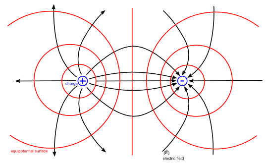
As a consequence of equipotential surfaces, electric fields (in a particular direction) are sometimes measured in units [V/m]. A strong electric field would thus result in a larger potential difference between two fixed points in space. A charged particle in this electric field would thus undergo greater acceleration. This acceleration would also mean a higher electric current between the two points.

This leads to the concept of electric breakdown. The electric breakdown of a material is the potential difference required to cause a rapid drop in resistance to current flow through that material. A related concept is the dielectric strength measured in [V/m]. This reduced resistance is in part a result of ionization of the material – spare ions are now available to conduct charge from one location to the other. The improved conductivity of the material can further result in a phenomenon known as coronal discharge whereby a steady current of charge leaks through the material after breakdown. Electrical breakdown is a particularly important characteristic of electrical insulators. 

10.5. Ohm’s Law

Given our knowledge of electric current, voltage and resistance its possible to derive Ohm’s Law. This derivation can be done with the following four equations:

Electromotive Force

\varepsilon =  V = \Delta V = V_b - V_a = - \int_{a}^{b}{\vec{E} \cdot d\vec{l}} \tag{23}

Conductivity

\sigma = \frac{\vec{J}}{\vec{E}} \tag{21}

Current Density

\vec{J} = \frac{I}{\vec{A}} \tag{17}

Resistance

R = \frac{l}{\sigma A} \tag{20}

Solving and substituting we get ohm’s law. In most electronic circuit related problems, ohm’s law is used as shown. It acts as a macroscopic law. 

Ohm’s Law

\varepsilon =  V = I R \tag{23C}

11. Magnetic Moment (m)

Electric fields and electric forces arise from the presence of electric monopoles. In the case of magnetism, to present day, no one has been able to discover magnetic monopoles. All magnets in existence today are magnetic dipoles. This makes a simple definition of magnetic force F_M quite tricky.   One approach to modeling this force, is to assume that magnetic monopoles exist and try to construct the equivalent of Coulomb’s law for magnetism (see Gilbert’s Model).  I won’t discuss this approach, primarily because I don’t have a lot of information about it. So let’s look at another approach.

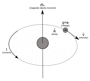
Magnetism arise from three atomic effects: Nuclear Spin, Electron Spin and Electron Orbital Motion. These effects lie in the realm of quantum mechanics. And, well, I don’t really understand quantum mechanics all that well. However, what I can say is that magnetic dipole moment, m is a measure of the contribution of these three effects to a material’s magnetic properties. This moment is typically defined in terms of electric current, I, and current loop area, A, as shown in the equation below (also see figure 13). We can also represent magnetic moment in a more arbitrary volumetric case where current distribution is more complex (i.e. current density J).

Magnetic Dipole Moment

\vec{m} = I \cdot {\vec{A}} \tag{24}

Magnetic Dipole Moment

\vec{m} = \frac{1}{2} \int{(\vec{r} \times \vec{J})\; dV} \tag{24A}

The magnetic moment is measured in units of:  [A m²]. The value r is the vector position pointing to the location of the volume element, dV and J current density at that location. 

12. Magnetic Fields (H, M and B)

I present to you for your consideration a solenoid and some arbitrary material suspended in free (empty) space (figure 14). This solenoid is composed of a wire wound around a cylinder and carrying a current.

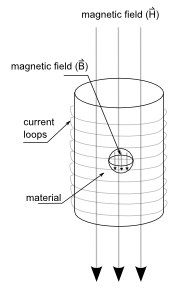
The current produces a magnetic field which passes through the suspended material. The magnetic field external to the material (generated by the solenoid) is called the H field or the magnetic field strength.  In-fact, it doesn’t matter what generates this field … as long as we understand that this external field is independent of the medium through which it is traversing. The H is measured in units of amperes per meter [A/m].

As the H field enters the suspended material, it is modified and an internal field is generated inside the material. This internal field is called the B field or the magnetic flux density. The B is measured in units of Tesla [T]. There is another component to this material response. One part of the response is a result of the external H field, the other is a result of the material’s intrinsic magnetization, M. The magnetization is measured in units [A/m]. Normally materials do not have any magnetization, however when they do, this magnetization is proportional to the external field (in the case of diamagnetic and paramagnetic materials – see equation 25) or a result of the intrinsic material properties themselves. In this intrinsic case we have to look at the magnetic dipole moment as a basis for computing the magnetization (equation 25a).  

Material Dependent Field

\vec{B} = {\mu}_{0} \cdot (\vec{H} + \vec{M}) \tag{25}

We can construct a representation of the relationship between these three materials using the formula below. The value μ₀ is known as the magnetic permeability of free space. This permeability represents a scaling factor for the external and magnetization field. Wait wait! I just realized a strange inconsistency in this argument – the magnetization of the object is a result of the intrinsic properties of the material … wouldn’t this mean that the material scaling is already taken into account? Or is the permeability a result of macroscopic material effects?

Paramagnets and diamagnets don’t have any intrinsic magnetization. In such cases, the magnetization of the material is proportional to the applied field as shown below in equations 26.  A quantity related to magnetic permeability of free space is that of relative permeability, μ_r. The relative permeability is specific to the material. This material’s specific response can also be represented by what’s known as the magnetic susceptibility, χ_M = μ_r – 1. Together the permeability of free space and the relative permeability of the material can be represented as μ=μ₀μ_r.  Utilizing the definition of magnetization for linear materials we see a simplified representation of the B field (equation 25a). 

Magnetization

\vec{M} = \chi_{\small{M}} \cdot {\vec{H}} \tag{26}

Material Dependent Field

\vec{B} = {\mu}_{0} \cdot (\vec{H} + \vec{M}) \tag{25}

\begin{aligned}
\vec{B} = & {\mu}_{0} \cdot (\vec{H} +  \chi_{\small{M}} \cdot {\vec{H}}) \\ \; \\
\vec{B} = & {\mu}_{0} \cdot (\vec{H} +   (\mu_r - 1)  \cdot {\vec{H}})
\end{aligned}

Material Dependent Field

\vec{B} = {\mu}_{0} \mu_r \cdot {\vec{H}} = \mu \cdot {\vec{H}}\tag{25A}

Ferromagnets may have an intrinsic magnetization. This magnetization doesn’t follow a linear relationship as shown in equation 26. So, what do we do? Well, for such scenarios an externally applied H field produces a non-linear response B field. This response is sometimes mapped as a hysteresis curve – I’ll discuss more about hysteresis towards the end of this article.

Now, going back to magnetization. If we consider the atomic scale behaviour of a material we can represent the magnetization of a material using a slightly different form (equation 27).

Magnetization

\vec{M} = \frac{N}{V} \cdot \vec{m} = \sum_{i}^{N}{\frac{1}{V} \cdot \vec{m}_{i}} \equiv \frac{1}{V}\cdot \vec{m} \tag{27} 

Notice that in the above equation the value N is a representation of the number of magnetic dipoles inside the material. Sometimes this number is combined with the magnetic moment as shown in the equivalence in the above equations. 

13. Magnetic Force and Torque (F_M, τ_M)

We see that for some current loop the magnetic force on that loop by some external field can be given in one of the following two ways:

Magnetic Force

\vec{F}_{\;\small{M}} = Q \cdot \vec{v} \times \vec{B} = \vec{J} \times \vec{B} \tag{27}

Magnetic Force

\vec{F}_{\;\small{M}} = \nabla (\vec{m} \cdot \vec{B}) \tag{27A}

Lets consider for an instant that a material is immersed in an external magnetic field, H. This external field will cause a material response B. In these equations, F_M is the force on the material, applied over the entire volume of the material. In the first representation, we need to link the concept of current (I, J), charge (Q) and velocity (v) from electrostatics to determine this force – essentially a link to the Lorentz force law. In the second representation we use the concept of magnetic moments. In practice, a solenoid with a known current and thus a known magnetic field, H can be used as a basis for determining a magnetic material’s magnetization (and moments). 

Given our earlier representation of moment, we can also define the torque experience by a magnetic material under an external magnetic field, B.

Magnetic Torque

\vec{\tau}_{\;\;\small{M}} = \vec{m} \times \vec{B} \tag{27B}

14. Lorentz Force Law

We saw, at the beginning of this article, an equation for the Lorentz Force Law. Here it is again, in case you forgot!

Lorentz Force Law

\vec{F} = \vec{F}_{\;\small{E}} + \vec{F}_{\;\small{M}} =  Q \cdot (\vec{E} + \vec{v} \times \vec{B}) = Q \; \vec{E} + \vec{J} \times \vec{B} \tag{5}

The law presents the relationship between electric and magnetic fields and their contribution to the total force in an electromagnetic system. 

15. Magnetic Flux (ϕ_M)

Like electric flux, magnetic flux is a scalar and is quite easy to define. The magnetic flux is measured in units of Tesla per meter squared [T/m²]. Sometimes this combined unit is known as the Weber [Wb].

Magnetic Flux through Surface 

{\phi}_{\small{M}} = \int_{S}{\vec{B} \cdot \vec{n} \cdot dA} = \int_{S}{\vec{B} \cdot \vec{dA}} \tag{28}

16. Gauss’ Magnetic Field Law 

I’ve re-iterated Gauss’ Magnetic Field Law in both integral and differential form in the equations below. This law is very similar to the electric field law and can be approached in much the same way, barring one exception. With magnetic particles there are no magnetic monopoles. Only dipoles. Meaning that a closed surface must by necessity have as many magnetic field lines coming into it as there are going out of it. The net flux passing through this surface is zero! Or alternatively, the divergence is zero. 

Gauss’ Electric Field Law

{\phi}_{\small{M}} = \oint_{S}{\vec{B} \cdot d\vec{A}} = 0 \tag{2}

\nabla \cdot \vec{B} = 0 \tag{2A}

17. Faraday-Maxwell Law and Kirchhoff’s Law 

Earlier when talking about EMF we noted the following relationship between voltage and electric fields.  Faraday discovered that a changing magnetic field can also induce a voltage.

Electromotive Force

\varepsilon = - \int_{C}{\vec{E} \cdot d\vec{l}} \tag{23}

The induced voltage is proportional to the rate of change of flux as shown below. The differential form can be derived from the integral form using Stoke’s Theorem.

Faraday’s Law

\varepsilon_{ind} = - \oint_{C}{\vec{E} \cdot d\vec{l}} = - \frac{\partial \phi_{\small{M}}}{\partial t} \tag{3}

\nabla \times \vec{E} = - \frac{\partial \vec{B}}{\partial t} \tag{3A}

In the event that the electric field in Faraday’s law is conservative, the law is known as Kirchhoff’s Law. However, conservative fields imply that the change in magnetic flux, ϕ_M must be zero!

18. Magnetomotive Force (F), Reluctance (R) & Hopkinson’s law

The magnetomotive force (MMF) is an analogue of electromotive force, but for magnetic fields. This force is denoted with the script letter, script F and defined as shown below:

Magnetomotive Force

\mathcal{F} = \int_{C}{\vec{H} \cdot d\vec{l}} \tag{29}

In an attempt to simplify, magnetic field calculations for electric machines, its useful to think in terms of magnetic circuits. These circuits are analogous to electric circuits. When talking about EMF, we know that electric charge is moving. In the case, of MMF, there are no moving magnetic charges. However, we can assume hypothetical magnetic charges. The magnetic flux, ϕ_M, then, is treated as this hypothetical current and follows similar rules to that of electric current. For instance, ϕ_M is additive at a nodal points.

Magnetic circuits also have a reluctance, script R. This reluctance is an analogue of resistance. Like resistance, reluctance obeys additive rules – e.g. reluctances in series add up. 

Reluctance

\mathcal{R} = \frac{l}{\mu A} \tag{30}

An equivalent of Ohm’s law is also possible with magnetic circuits. This equivalent is called Hopkinson’s law and is shown below. Despite the apparent similarities between magnetic and electric circuits, though, its important to remember that the relationships are largely superficial and care should be taken during analysis. 

Hopkinson’s Law

\mathcal{F} = \phi_{\small{M}} \mathcal{R} \tag{31}

19. Ampere-Maxwell Law

The Ampere-Maxwell law is defined below. The law appears in many forms in literature, but regardless of form takes into account the reversibility of electromagnetic induction. Not only does a changing magnetic field (B) induce an emf (ε_ind​) but also, a changing electric field, (D) induces a mmf (script F).

Ampere – Maxwell Law

\mathcal{F_{ind}} = \oint_{C}{\vec{H} \cdot d\vec{l}} = \int_{S}{\left(\frac{\partial \vec{D}}{\partial t} + \vec{J}\right) \cdot d\vec{A}} \tag{4}

\nabla \times \vec{H} = \frac{\partial \vec{D}}{\partial t} + \vec{J}\tag{4A}

The law comes in various forms. We can easily take the integral form and represent it in terms of flux and current. Note that the surface, S, is the cross-sectional surface through which the electric current is flowing – if we consider a solenoid, the integral ∫_S​J⋅dA reduces down to N⋅I with N being the number of loops in the coil. 

Ampere – Maxwell Law

\mathcal{F_{ind}} = \oint_{C}{\vec{H} \cdot d\vec{l}} = \frac{\partial \phi_{\small{E}}}{\partial t} + I \tag{4B}

20. Hysteresis, Coercivity, Remenance, Saturation 

Figure 10 below demonstrates a property called hysteresis, a property which only exists in ferromagnetic materials. The hysteresis curve below models the response of a ferromagnetic material to an externally applied field, H. Initially the material has never been exposed to a magnetic field. This leads us to position (a) in the curve. As the external magnetic field increases, magnetic domains in side the material align with and reinforce the external field. If we were to measure the field, B inside the material we would see it rise along with H along what’s known as the virginal curve. Yes, yes, I know … physicists have dirty minds …

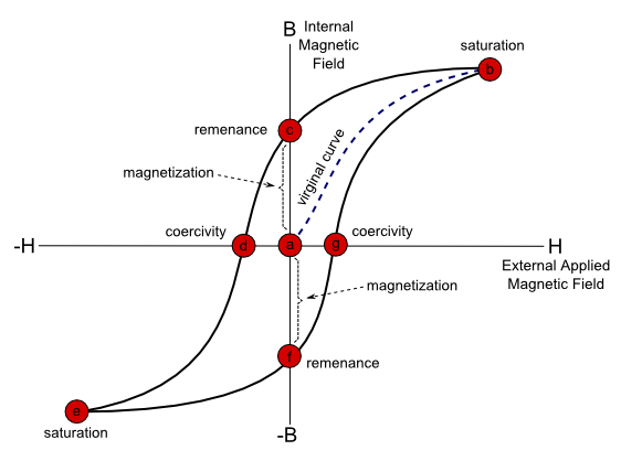
At some point, all the domains and dipoles in the ferromagnetic material have been aligned with the external H field. At this point, (b), the material is said to be saturated and the B increases linearly with the external applied field, H … so the material starts to behave more like a diamagnetic or paramagnetic material.

At this point if we remove the external field, the internal magnetic field drops off to point (c) in the curve. At this point the material has become magnetized and is said to have a magnetic remanence. We can link this to the idea of magnetization . The net magnetic dipole moments of the material without an external field are non-zero at this remanence point.

In order to remove this remnant magnetism we must now apply a field in the opposite direction … so if we continue, the B, will continue to drop and at some point will reach a value of zero. This point, (d), is known as the coercivity of the material. At this point continuing to increase H in the negative direction eventually leads to saturation again (point (e)). And again the material starts responding linearly to increases in H. We can then continue this process going through points (f) and (g) by changing the direction of the external field again.

References

1. Feynman Lectures in Physics.; 1963.