
In the world of electrical machines, we stuffy engineers like to wax intellectual and spout all sorts of age old wisdom from all sorts of dusty old books. Today I’m going to dust off some books and talk about the Newton-Raphson Numerical Method for estimating equation roots. This is a key method that many Finite Element Analysis (FEA) tools use to calculate magnetic fields. The truth is, as engineers, we use FEA all the time, but very few of us really understand the theory or how it all works. This is my first attempt to remedy that particular situation. But be patient! I’m only a beginner too! 🙂
As someone starting out in the field of electromagnetics one of the questions I had always asked myself is “how do we actually compute the bloody magnetic field at a particular position in space!” … normally there are far more explicit expletives … but I’ll spare, you, dear reader, the anguish.

Today, I’m going to try to answer that question with rigorous mathematics. You see, ultimately, what we have is a bunch of equations … call them Maxwell’s Equations plus and a sprinkling of a few other convenient little nuggets of equations … and our goal is to solve these equations for all the variables. Things are complicated by the fact that the variables themselves are functions of space and time. I’m going to use one particular approach to formalize the computation of approximate magnetic fields and the like for every point in space. Of course, because space is continuous and there are an infinite number of points, the first step is to discretize the space into finite elements and then perform the analysis or computation on these elements. Hence the name Finite Element Analysis (FEA).
The particular method that I’ll focus on as a first step to FEA and the estimation of magnetic fields is called the Newton-Raphson Method. Let’s go ahead and start our discussion!
Newton-Raphson Method for Solving Systems of Equations
Newton’s Method is a technique for finding the roots of an equation through successive approximation [1] [2]. Interesting fact, even though this method is called Newton’s Method, a variation of it was apparently discovered around 700BC by the Babylonians. Good ol’ Babylonians!
The roots are the locations where a particular function intercepts the x axis – i.e. the values of x that satisfy the equation:
f(x)=0
We’ve all done this analytically for equations like:
x^2 + 2x + 1 = 0
where the root is x=-1, for instance. Of course some equations are far far more difficult and a purely analytical solution can’t be found easily. In such cases, we use Newton’s method and start off with an initial guess for our x-intercept or root.
This is successively and iteratively refined until we can get close enough to our actual root for our particular application. The Newton-Raphson method is another name sometimes used for Newton’s method.
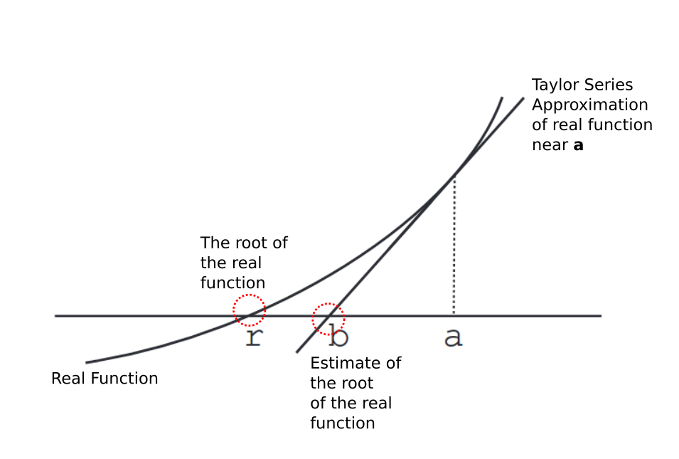
Now Newton’s method is actually based on Taylor series approximations. You may have this vague inkling of a memory from your undergraduate class, where the Taylor series approximation was given for a single variable function, f(x) at some value x=a as shown below. The function p(x) is the nth order Taylor series approximation, i.e. p(n)(x).
Single Variable Taylor Series
\begin{aligned}
p_{\small{(n)}}(x) \approx f(a) &+ \frac{1}{1!}f'(a)(x-a) + \frac{1}{2!}f''(a)(x-a)^2 \\ &+ \frac{1}{3!}f^{(3)}(a)(x-a)^3 +\;\;...\;\;+ \frac{1}{n!}f^{(n)}(a)(x-a)^n
\end{aligned}
The Taylor series here tries to find an accurate approximation of the function near the point x=a. As we get further and further from this point the value becomes less accurate. The error between our approximation for the Taylor series and the real function value can be represented as shown below by r(n)(x) and e(n)(x). In-fact, we can come up with an exact representation of the original function by rearranging this error function.
Lagrange Remainder (via the Mean Value Theorem)
r_{(n)}(x)=f(x)-p_{(n)}(x)=\frac{f^{(n+1)}(c)}{(n+1)!}(x-a)^{(n+1)}\\ \; \\
\;\;\;\;\;\;\;\;\;\;\;\;\;\;\;\;\;\;\;\text{with}\;\;c\in[a,x]\;\;\text{or}\;\;c\in[x,a]\;\;\text{so}\;\;r_{n}(x)\;\text{is max.}
Lagrange Error
e_{(n)}(x)=|r_{(n)}(x)|Single Variable Taylor Series with Remainder
\begin{aligned}
f(x)&=p_{(n)}(x) + r_{(n)}(x)\\
&=f(a) + \frac{1}{1!}f'(a)(x-a) + \frac{1}{2!}f''(a)(x-a)^2 \\
&\;\;\;+ \frac{1}{3!}f^{(3)}(a)(x-a)^3 +\;\;...\;\;+ \frac{1}{n!}f^{(n)}(a)(x-a)^n + r_{(n)}(x)
\end{aligned}
Looking at the remainder, we note that c is some value (we don’t know what value) such that c is between [a,x]. That, of-course, doesn’t really help. Basically, the problem is that you cannot know the error, e(n)(x), exactly because the actual function, f(x) is unknown. But what you can do is put an upper bound on this error so that at least we have some idea of how good our approximation is likely to be. When computing the upper bound we can choose our value c such that the overall error.
e_{(n)}(x) \leq |r_{(n)}(x)| \;\;\;\text{for a known order}\;n \;\text{and value}\; xA major problem with the Taylor series approach is the fact that the function and its various nth order derivatives must be differentiable. But this isn’t always the case! Sooooooo …. what do we do? We use a finite difference approach to estimating the derivative using what’s known as the Secant Method! But I’ll discuss that all later! For now let’s continue with the Taylor series.
But one variable functions are hardly anything special. Furthermore the above definition assumes that the function, f(x) is a scalar – this may not be true. So we can expand the series to multivariate vector equations too. So let’s suppose we’ve got a multivariate vector function F(X) as shown below with X= [x1, x2, …. xq]. The value q is simply the number of variables that the function F depends upon.
\vec{F}\;(\vec{X})=\left[\begin{matrix}f_1(x_1, x_2,\;...\;, x_q) \\ f_2( x_1, x_2,\;...\;, x_q) \\ \vdots \\ f_m( x_1, x_2,\;...\;, x_q)\end{matrix}\right]With this multivariate representation we can construct a Taylor series as shown below. Again, as before, the approximation P(n)(X) is the nth order Taylor series for the function F(X), with X=[x1, x2, …, xq] near some known point, A=[a1, a2, … , aq].
Multivariable Taylor Series
\begin{aligned}
\vec{P}_{\;(n)}(\vec{X}) \approx &\vec{F}\;(\vec{A}) + \frac{1}{1!}\vec{F}  '(\vec{A})(\vec{X}-\vec{A}) + \frac{1}{2!}\vec{F}\;''(\vec{A})(\vec{X}-\vec{A})^2\;\;\;\;\\&+ \frac{1}{3!}\vec{F}\;^{(3)}(\vec{A})(\vec{X}-\vec{A})^3 +\;\;...\;\;+ \frac{1}{n!}\vec{F}\;^{(n)}(\vec{A})(\vec{X}-\vec{A})^n
\end{aligned}
Multivariable Taylor Series (differential operator notation)
\begin{aligned}
\vec{P}_{\;(n)}(\vec{X}) \approx &\; \vec{F}(\vec{A})+ \frac{1}{1!}D\vec{F}\;(\vec{A})(\vec{X}-\vec{A})+\frac{1}{2!}D^2\vec{F}\;(\vec{A})(\vec{X}-\vec{A})^2 \\ &+ \frac{1}{3!}D^3\vec{F}\;(\vec{A})(\vec{X}-\vec{A})^3 + \;\;...\;\;+ \frac{1}{n!}D^{n}\vec{F}\;(\vec{A})(\vec{X}-\vec{A})^n
\end{aligned}
Along with these representations we can also start to look at the nth order error and remainder/residual. These are defined below for the multivariate case.
Lagrange Remainder
\vec{R}_{\;(n)}(\vec{X})=\vec{F}\;(\vec{X})-\vec{P}_{\;(n)}(\vec{X})=\frac{\vec{F}^{\;\;(n+1)}(\vec{C})}{(n+1)!}(\vec{X}-\vec{A})^{\;(n+1)}\\
\; \\ \;\;\;\;\;\;\;\;\;\;\;\;\;\;\;\;\;\;\;\text{with}\;\; \vec{C}\in[\vec{A},\vec{X}]\;\;\text{or}\;\;\vec{C}\in[\vec{X},\vec{A}]\;\;\text{so}\;\;\vec{R}_{\;n}(\vec{X})\;\;\text{is max.}
Lagrange Error
\vec{E}_{\;(n)}(\vec{X})=|\vec{R}_{\;(n)}(\vec{X})|Multivariable Taylor Series with Remainder
\begin{aligned}
\vec{F}(\vec{X}) = & \;\vec{F}(\vec{A}) + \frac{1}{1!}\vec{F}'(\vec{A})(\vec{X}-\vec{A})+ \frac{1}{2!}\vec{F}''(\vec{A})(\vec{X} -\vec{A})^2 \\ &+ \frac{1}{3!}\vec{F}^{(3)}(\vec{A})(\vec{X}-\vec{A})^3 +\;\;...\;\;\\ &+ \frac{1}{n!}\vec{F}^{(n)}(\vec{A})(\vec{X}-\vec{A})^n + \vec{R}_{n}(\vec{X})
\end{aligned}
Now here’s where things become tricksy! How do we compute the first and second derivatives, etc. of a multivariate vector function? … The first derivative of
\vec{F}(\vec{X}), \; \text{call it}\; \vec{\mathcal{J}}(\vec{X})=\vec{F}'(\vec{X})can be represented in the form known as the Jacobian Matrix, J. Likewise the second derivative,
\vec{\mathcal{H}}(\vec{X})=\vec{F}''(\vec{X})can be represented in the form commonly known as the Hessian Matrix, H. So let’s start with those two!
Jacobian Matrix
\vec{\mathcal{J}}(\vec{X})=\vec{F}\;'(\vec{X})=\left[\begin{matrix}\frac{\partial f_1}{\partial x_1} & \frac{\partial f_1}{\partial x_2} & \dots & \frac{\partial f_1}{\partial x_q} \\ \frac{\partial f_2}{\partial x_1} & \frac{\partial f_2}{\partial x_2} & \dots & \frac{\partial f_2}{\partial x_q} \\ \vdots & \vdots & \ddots & \vdots \\ \frac{\partial f_m}{\partial x_1} & \frac{\partial f_m}{\partial x_2} & \dots & \frac{\partial f_m}{\partial x_q} \end{matrix}\right]Hessian Matrix
\vec{\mathcal{H}}_{f_1}(\vec{X})=f_1''(\vec{X})=\left[\begin{matrix}\frac{\partial f_1}{\partial x_1 \partial x_1} & \frac{\partial f_1}{\partial x_1 \partial x_2} & \dots & \frac{\partial f_1}{\partial x_1 \partial x_q} \\ \frac{\partial f_1}{\partial x_2 \partial x_1} &  \frac{\partial f_1}{\partial x_2 \partial x_2} & \dots &  \frac{\partial f_1}{\partial x_2 \partial x_q} \\ \vdots & \vdots & \ddots & \vdots \\ \frac{\partial f_1}{\partial x_q \partial x_1} & \frac{\partial f_1}{\partial x_q \partial x_2} & \dots & \frac{\partial f_1}{\partial x_q \partial x_q} \end{matrix}\right]\\ \; \\ \; \\

\vec{\mathcal{H}}_{f_2}(\vec{X})=f_2''(\vec{X})=\left[\begin{matrix}\frac{\partial f_2}{\partial x_1 \partial x_1} & \frac{\partial f_2}{\partial x_1 \partial x_2} & \dots & \frac{\partial f_2}{\partial x_1 \partial x_q} \\ \frac{\partial f_2}{\partial x_2 \partial x_1} & \frac{\partial f_2}{\partial x_2 \partial x_2} & \dots & \frac{\partial f_2}{\partial x_2 \partial x_q} \\ \vdots & \vdots & \ddots & \vdots \\ \frac{\partial f_2}{\partial x_q \partial x_1} & \frac{\partial f_2}{\partial x_q \partial x_2} & \dots & \frac{\partial f_2}{\partial x_q \partial x_q} \end{matrix}\right]\\ \; \\
\;\;\;\vdots\\ \; \\
\vec{\mathcal{H}}_{f_m}(\vec{X})=f_m''(\vec{X})=\left[\begin{matrix}\frac{\partial f_m}{\partial x_1 \partial x_1} & \frac{\partial f_m}{\partial x_1 \partial x_2} & \dots & \frac{\partial f_m}{\partial x_1 \partial x_q} \\ \frac{\partial f_m}{\partial x_2 \partial x_1} & \frac{\partial f_m}{\partial x_2 \partial x_2} & \dots & \frac{\partial f_m}{\partial x_2 \partial x_q} \\ \vdots & \vdots & \ddots & \vdots \\ \frac{\partial f_m}{\partial x_q \partial x_1} & \frac{\partial f_m}{\partial x_q \partial x_2} & \dots & \frac{\partial f_m}{\partial x_q \partial x_q} \end{matrix}\right]
The Jacobian and Hessian matrices for our arbitrary m dimensional (directional) function with q variables, F(X) are defined above. I’m not going to go into higher order derivatives at the moment as this is a bit more complicated and, frankly, I don’t really know how to easily express them. But what I can do is re-write our Taylor series using the Jacobian and the Hessian matrix as follows:
\vec{P}_{\;(2)}(\vec{X}) \approx \vec{F}\;(\vec{A}) + \frac{1}{1!}\vec{\mathcal{J}}(\vec{A})(\vec{X}-\vec{A}) + \frac{1}{2!}\vec{\mathcal{H}}(\vec{A})(\vec{X}-\vec{A})^2So let’s get back to Newton-Raphson and bring it all together to actually solve some equations! So now that we have a Taylor series for our multivariate vector function, let’s suppose that we can represent our particular function as an equation of the form, F(X)=0. This might be difficult to solve for the roots, X. This is where the Taylor series comes in. We can replace our F(X) with a linear or quadratic approximation, either
\vec{P}_{\;(1)}(\vec{X})\; \text{or} \; \vec{P}_{\;(2)}(\vec{X})\;System of Equations For the Newton-Raphson Method
\begin{aligned}
\vec{F}\;(\vec{X}) = \vec{0} \implies \left\{\begin{array}{l}f_1(x_1,x_2,\;...\;,x_q) = 0 \\  f_2(x_1,x_2,\dots,x_q) = 0  \\ \;\;\;\; \vdots \\  f_m(x_1,x_2, \dots, x_q) = 0 \end{array}\right.\\ \; \\ \; \\

\vec{F}\;(\vec{X}) \approx  \vec{P}_{\;(1)}(\vec{X}) = \vec{0} \implies \left\{\begin{array}{l}p_1(x_1,x_2,\;...\;,x_q) = 0 \\  p_2(x_1,x_2,\dots,x_q) = 0  \\ \;\;\;\; \vdots \\  p_m(x_1,x_2, \dots, x_q) = 0 \end{array}\right.
\end{aligned}
Now. How do we actually solve this system of equations? That, my friends, requires a bit more work! So, the first thing we note is that for us to be able to solve a system of equations the number of unknowns must be at most equal to the number of equations available to us. This means that m >= q. Further, to start the process off, we need to make a good initial guess of our variable, X. Let’s call this initial guess A=X0. Furthermore let’s consider a first order Taylor series approximation P(1)(X). From this we can construct a refined estimate, X1 of our root as shown below.
Estimate Root
\begin{aligned}
\vec{F}\;(\vec{X}) \approx \vec{P}_{\;(1)}(\vec{X}) =  \vec{F}\;(\vec{A}) + \frac{1}{1!}\vec{\mathcal{J}}(\vec{A})(\vec{X}-\vec{A}) = \vec{0}\\
\end{aligned}
\begin{aligned}
\text{Let}\;\;\vec{A}=\vec{X}_{\;0}\;\;\text{and}\;\;\vec{X}=\vec{X}_{\;1}\\ \; \\
\vec{F}\;(\vec{X}_{\;0}) + \vec{\mathcal{J}}(\vec{X}_{\;0})(\vec{X}_{\;1}-\vec{X}_{\;0}) = \vec{0}\\ \; \\
\vec{X}_{\;1} = \vec{X}_{\;0} - \vec{\mathcal{J}}(\vec{X}_{\;0})^{-1}\vec{F}\;(\vec{X}_{\;0})
\end{aligned}\begin{aligned}
\text{Let}\;\;\vec{A}=\vec{X}_{\;1}\;\;\text{and}\;\;\vec{X}=\vec{X}_{\;2}\\ \; \\
\vec{X}_{\;2} = \vec{X}_{\;1} - \vec{\mathcal{J}}(\vec{X}_{\;1})^{-1}\vec{F}\;(\vec{X}_{\;1})
\end{aligned}\text{Let}\;\;\vec{A}=\vec{X}_{\;2}\;\;\text{and}\;\;\vec{X}=\vec{X}_{\;3}\\ \; \\
\vec{X}_{\;3} = \vec{X}_{\;2} - \vec{\mathcal{J}}(\vec{X}_{\;2})^{-1}\vec{F}\;(\vec{X}_{\;2})\\ \; \\
\;\;\;\vdots\\ \; \\
\text{Continue until error is minimized}Eventually, repeating and refining the root computation can eventually lead to convergence to a single value. Determining the degree of convergence that is acceptable for our particular problem can be set by the user by bounding the error between consecutive computations of the root.
The question is: How do we determine our stopping criteria? One way is to look at the relative change of our estimated root. If the root changes only by a small enough amount on consecutive iterations, then we can say that we’ve reached convergence. Of-course, we, as the user, must determine what that small enough amount is – sometimes known as a tolerence, T. A simple way of doing this is to define an error condition, α, as follows. We stop when the α is less than or equal to our tolerence, T.
\alpha = | X_{i} - X_{i-1} | \leq T \; \text{given a tolerence},\; T\; \text{and for some iteration}, i.At this point, you might be wondering why I even discussed error bounding in our earlier discussion about remainders. Well, the truth is that we have to figure out exactly how good our initial guess, X0 has to be in order for Newton’s method to converge .
Addressing Failures of Newton’s Method
One of the primary failures of Newton’s Method lies in the fact that the system of equations in question must be differentiable. This is not always the case. A variation to avoid this issue is the Secant Method which uses finite differences rather than differentiation for the Taylor series approximation.
Newton’s method also explicitly requires that the initial guess be fairly good. A poor guess can mean that the method simply cannot converge to an appropriate root. In some cases the convergence can be an oscillation between two or more values. The reason behind this poor convergence under poor initial guess is that we make the assumption that the quadratic hessian term in our Taylor approximation is small enough that it can be deleted. And also that the same is true for the higher order derivatives. This would only be true when our initial guess is close to the actual root. Another method, sometimes known as the bi-section method is used as an alternative – this method never fails, but tends to operate much much more slowly than Newton’s method.
Another final failure of the method occurs if our derivative near our actual root is close to zero. Not completely sure, but I suspect this is because estimating the root via Newton’s method requires a division by the derivative. If the derivative is close to zero our root estimates can become very very big and eventually undefined.
A thing to note is that there may be multiple roots in our equation F(X)=0 which means that there is no unique solution to the equation. In order to get all the solutions, we would therefore have to start Newton’s Method at multiple different initial guesses, with each guess being near one of the roots. This is problematic since we don’t really know how many solutions to expect from our equation and hence how many roots exist.
Other variations of Newton’s Method exist to overcome these problems. Among them is the Quasi-Newton Methods, of which The Secant Method is one of. Another method is the Broyden-Fletcher-Goldfarb-Shanno (BFGS) Method. I’ll discuss these perhaps in another article.
References
- Anstee R. The Newton-Raphson Method. 2006. Available from: https://www.math.ubc.ca/~anstee/math104/104newtonmethod.pdf
- Kuczmann M. Newton-Raphson Method in Nonlinear Magnetics. 2008. Available from: https://maxwell.sze.hu/docs/h40.pdf
- Godfrey Kneller. Painting of Sir Isaac Newton. 1702. https://commons.wikimedia.org/w/index.php?curid=6364764