Python & PID Controlled Magnetic Levitation

Siraj Sabihuddin

A scientist and engineering doing a quick and dirty implementation of a simple magnetic field simulation of levitation by induction and PID airgap control

Donate

Shop

Contact

It can be tough to find detailed information about electromagnetic simulations online – at least as things stand in the present internet. Where information is present it is provided in some standard form as outlined by textbooks and it is not always immediately apparent how this textbook knowledge can be translated into implementations. In this article, I build a very simple and maybe inaccurate PID control system that very superficially pretends to run on a microcontroller. To support this, since I don’t have a real system to test on, I outline a very quick and dirty approach to modeling electromagnetic levitation of a set of coils above a track using python and a recently developed package: Magpylib [1][2].

1. Introduction

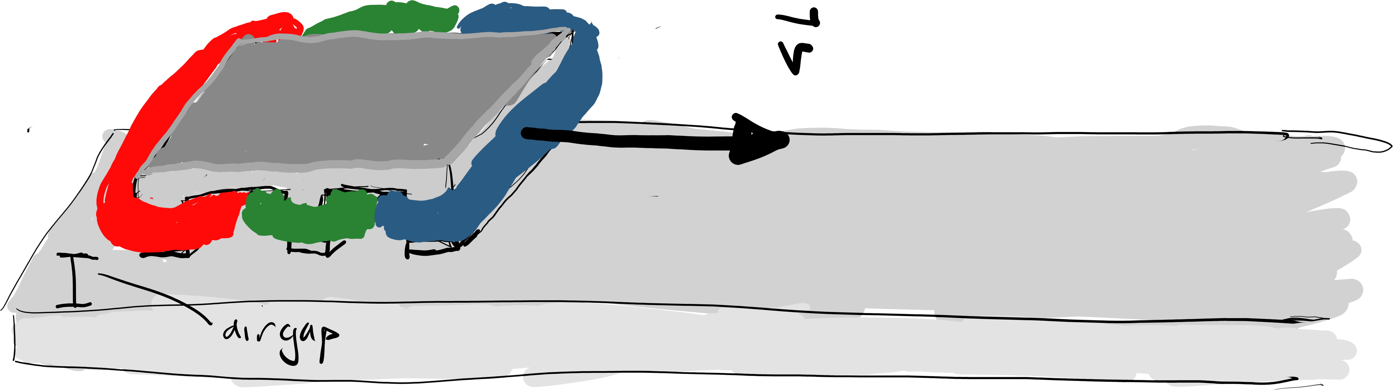
So recently, I had a bit of time to work on a problem that landed on my plate. That of producing a PID controlled approach to levitating a series of coils above a fixed magnetic plate. The idea here is to maintain the air gap in the system of coils floating above a track. This is essentially the beginning of a Linear Induction Machine (see the figure below – figure 1). However, in my case I am not at present interested in the translation movement of the coils, but only in the air gap distance and its control. The current in the coils is a filtered and amplified voltage provided, in theory, by a microcontroller PWM signal.

2. Magnetic System Overview

Since I haven’t got a real system to test on, I will create a quick and dirty implementation. The geometry for this simple machine is assumed to be as shown in the diagram above (figure 1) and below (figure 2).

Using magpylib [1][2], the above diagram can be modeled in python. This modeling is shown in the code below.

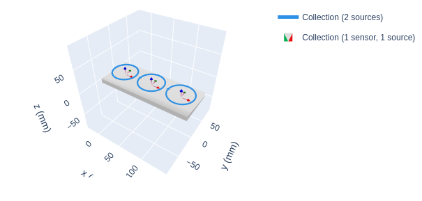
Once modeled a simple way of displaying the model is using python graphing features. An example of code for this is shown below. The code first creates a model. Here the model consists of three coils of diameter D. These coils are initialized with a moving path going through a z-direction (vertical) translation away from the track. This path is used for computation of B-Fields later on in the code. A layout is used to assign x and y and z axis labels and the like.

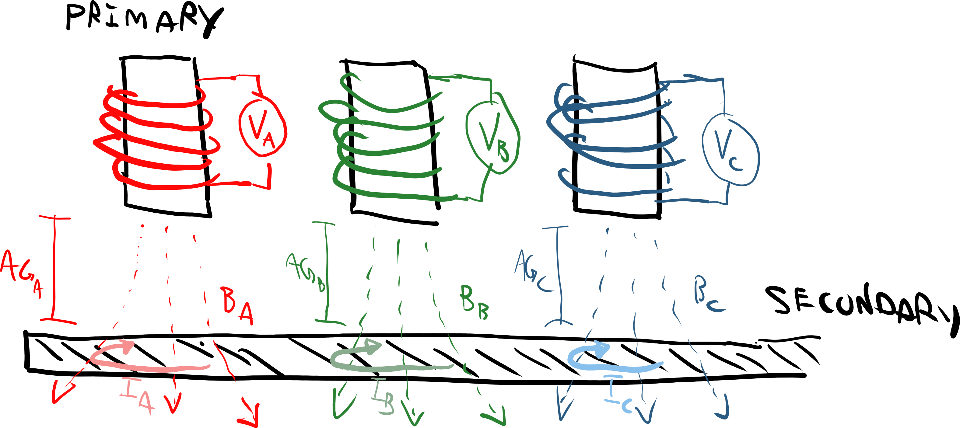
The resulting output of this code is shown in figure 3 below. Here the three coils are grouped into a single collection called the primary (containing three loop current sources) and the secondary (containing a zero magnetization bar magnet and another set of three sensors to measure the B-field). Note that these collection of three sensors are shown as a single source collection.

3. Voltage Source

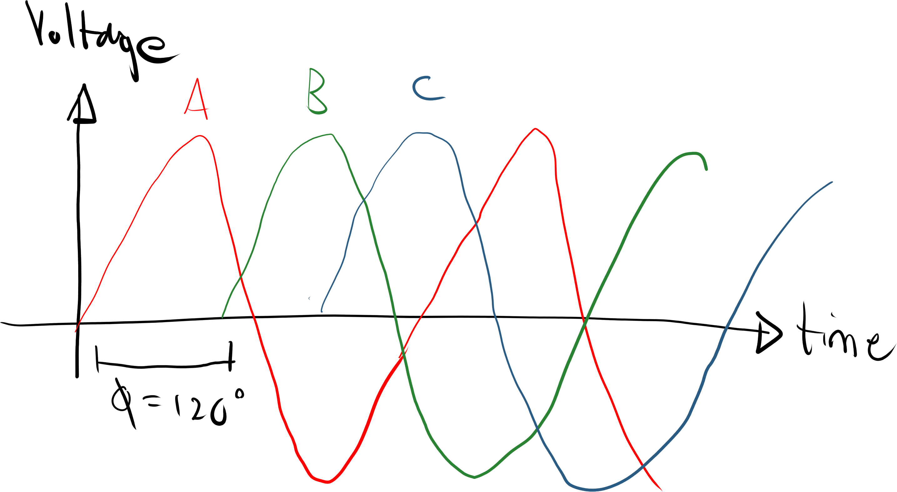
As shown earlier I assume that that the machine consists of three phase coils, A (0), B (1), C (2) each of which is independent from the other. In a typical induction machine you would want the coils to each received a voltage signal that is 120 degrees out of phase with the previous as shown in the figure 4 below. Where the translation velocity needs control the frequency of waveform would change for the linear induction machine.

To achieve this phase shifted waveform across the three coils a separate driver (see block diagram in figure 5) might be used to drive the voltage of each coil. Here a microcontroller might be used to produce a PWM waveform that is averaged, filtered and then amplified to drive the coil. The PWM needs to be sufficiently high in frequency as to allow smoothing without compromising on the ability to produce an oscillating voltage waveform at the coil location. In my case I assume that the coils are behaving as one and that each coil receives the same phase angle as all other coils. In essence we should be able to drive them with a single driver in practice.

This approach of using a single voltage waveform to drive three coils only allows control of the air gap between the primary (coils) and secondary (track) as a unified whole. This means that any pitch angle resulting from uneven mass distribution in the primary or any imperfections in the coils cannot be adjusted for.

In order to create an induced magnetic field in the track, it is necessary to generate a changing magnetic field. This changing field results in an induced current in the track. The way it is achieved is through a changing voltage across the coils of the primary. Typically a smooth voltage waveform, such as a sine wave, is preferred as it presents unknown transients resulting from discontinuities in the change in voltage on the coil.

Sine wave calculations in a small microcontroller (MCU) can have some difficulties. Many such small MCUs are not equipped with a floating point unit and so floating point approximations must be emulated in the firmware. Such emulation comes with a processing and potentially memory cost. An approximation of a sine wave can reduce this cost. For instance the use of a triangle wave function instead. Below is an example of a python function, triangle(t, ph, T), that produces a triangle wave that has as input the time, t, at which the value should be produced, the phase angle, ph, and the period, T, of the waveform.

The above code generates an output value between -1 and 1. In practice, the microcontroller will not directly output this value. And in some sense, I’m only paying lip service to the MCU’s capabilities as the triangle wave function itself generates a floating point output. In truth, a triangle wave approximation with an 8 or 16 bit MCU could perhaps be done more effectively. I’ll leave this as an exercise for later.

A PWM representation of this value will be output to produce a simulated Digital to Analogue conversion (DAC). If by some circumstance, a DAC is present, we would need to make some adjustments to the voltage waveform to fall between the 0 to 5 volt output range of the microcontroller anyway.

Assuming a PWM approach, we can take this triangle wave and determine the duty cycle of a PWM waveform. This is the percentage of time that the output of the microcontroller is in the ON (5 volt) state v.s. the OFF (0 volt) state. An example function to convert this triangle wave into a PWM wave is shown below.

In practice, the PWM output will have a bit resolution. This bit resolution can be simulated by the function voltage(val, bits, max). The bits variable limits the resolution of any function value input into this function, while the max variable provides a scaling.

We can feed the triangle wave function into a PWM output (functions: pwm() and voltage()) to get the equivalent triangle wave output as shown in the code below:

Notice that in figure 6, we see in red, the original triangle wave from function triangle(t, ph, T), while in green we see an approximation of what that waveform would look like if a 4 bit PWM output was smoothed by some low pass filter – this corresponds to the function: voltage(triangle(t,ph,T),bits,max). We can represent this approximated triangle wave using the pwm(t, value, period, max) function as shown in blue.

4. Coil & Track Fields

Since, I don’t have a real system, I assume that the coils can be represented as a single turn with a fixed resistance – i.e. no frequency response characteristics of the coil. This means that the voltage source can be controlled to achieve variable current to the coil.

I assume that coils are decoupled from each other as well and that no linking flux exists. The resistance of the track that produces the induced magnetic field is assumed to be fixed as well. In practice, as the changing B-field generated by the coil (primary) intersects the track (secondary), the induced voltage will be met with the resistance of the track. This resistance then limits the current induced and the resulting response B-field. I assume that this resistance is low and fixed (and that no frequency response issues exist) and thus the resulting current is decoupled from the frequency of the changing magnetic field or the specific lamination (or lack there of) of the track.

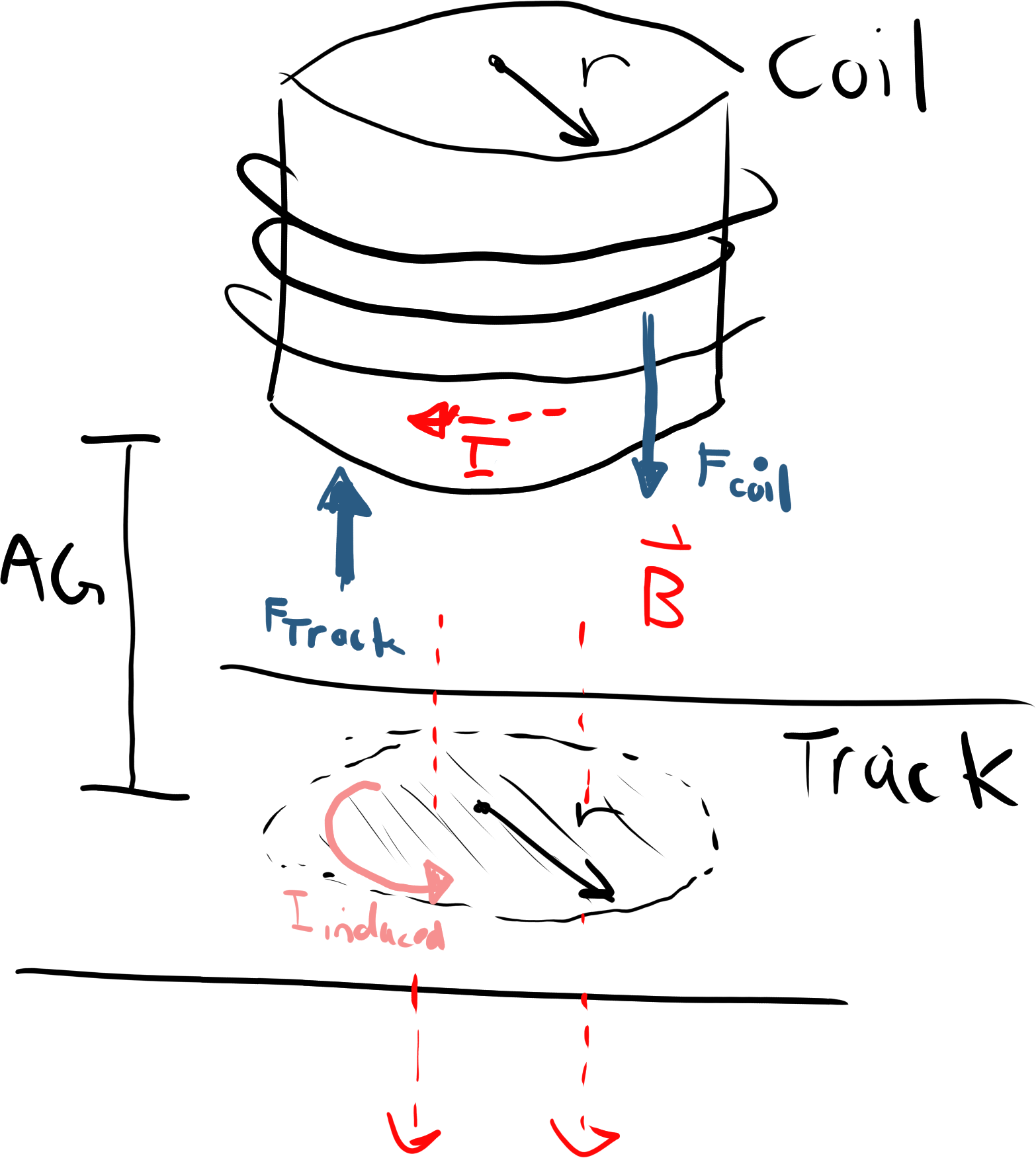
Finally, I also make an additional assumption. The B-field generated by the coil onto the track at some air gap distance AG, drops off as it would in air (i.e. relative permeability of 1). I assume this B-field is completely collimated – i.e. no leakage or spread of the field occurs in the air gap region. This therefore means that the B-field in the shadow region produced by the coil on the track is constant and uniform. It therefore makes calculation of the flux (Φ) simple. The area through which the B-Field passes is simply then πr², where r is the radius of the coil. In simulation I can thus measure the B-field at a single point on the track under the coil and use it with the shadow area (projection onto track) to compute this flux, Φ.

5. Force Calculations

I assume that each of the three coils comes with a single air gap sensor to measure the relative position of the primary (coil) assembly to the secondary (track). This could be an inductive sensor or laser sensor. Since, I’m assuming that no pitch control is present, the average of these three sensor values then becomes used as a single representation of the air gap.

For the purposes of simulation in python, I assume that the model shown in figure 3 and figure 7 is the geometry and respective simplification for computing the force. As in figure 7, we can now compute an estimate of the force exerted by the track on the coils as shown in steps 1 to 8 below:

\begin{align}F_{track} &= J_{track}(x,t) \times B_{coil}(x,t)\\ &= I_{track}(x,t) B_{coil}(x,t) sin(90)\\ &= \frac{V_{track}}{Z_{track}} B_{coil}(x,t)\\ &= \frac{d\phi_{coil}(x,t)}{dt} B_{coil}(x,t)\\ &= B_{coil}(x,t) \frac{d(\int{B_{coil}(x,t){dA}_{track}})}{dt}\\ &= B_{coil}(x,t) \frac{d}{dt}(B_{coil}(x,t)A_{track})\\ &= B_{coil}(x,t) \frac{d}{dt}(B_{coil}(x,t)\pi r_{coil}^2)\\ &= \pi r_{coil}^2 B_{coil}(x,t) \frac{d(B_{coil}(x,t))}{dt}\\\end{align}

In the above formula, I have used the induced track current J_track or I_track. This current is estimated by the changing flux dΦ_coil/dt presented at the location of the track by the particular coil. I assume that the B-field, B_coil produced by the primary coil of each phase is approximately uniform across the shadow produced by that coil on the track (the projection). This is of-course not the case in a real system. I’ve done this for expediency. The finalized equation (no. 8) and python code (as below), can, as a result be considerably simplified.

In order to compute the force, we can now utilize the function: force(b0, coils, sensors) with our magpylib geometry (coils, sensors) and an initial B-field (b0). This is used as below:

Notice that thus far we are computing the force per coil phase over a z-direction path from 0 to some ZMAX value. Note that the z-direction positions are, for the purposes of simplicity, iterated over whole number values in mm. This means that there is no fractional mm value such as 2.86 or 3.45, only whole numbers such as 2 and 3. This necessarily adds an additional error in our magnetic field and force simulation especially given the non-linear nature of the magnetic field. But I hope that this articles objective of a quick and dirty approach will be sufficient to justify this approach to the reader. In the next step we will compute the air-gaps between each coil phase and average them for use in PID control. The path will be used for a quick estimate of equilibrium position.

6. Equilibrium Airgap

At this stage, now that we can compute the B-field and force field we need to simulate the air gap sensor. In practice, this isn’t really necessary if a real system is available as it would, presumably, have an inductive or laser air gap sensor mounted on it. However, to verify our PID controller is functioning to correctly position the primary coils at a fixed position and air gap on top of the track, this step is helpful.

As we saw in section 2 of this article, we used magpylib to create a path over which we move the primary coils (see code below). We compute the force in section 5 over all coils and all positions in this path for every time, t, of the simulation. Now we know that our real system will have a fixed mass (MASS) and gravitational acceleration (G). This means that we can estimate the total force due to gravity of each coil as 1/3rd of all coils combined.

This approach means that we simply need to find the force balance between the magnetic force on each coil generated from the track and the force of gravity exerted on each coil such that F_g(coils) = F_track(coils). Unfortunately, a simple comparison won’t be possible between our force matrix F[] (in the code) and this F_g value since the F[] matrix is computed at discrete positions (upto ZMAX) in space. A very simple approach to solving the equation F_g(coils) = F_track(coils) for the equilibrium position is to utilize a nearest neighbour technique. Here we can compare the F_g value to every positional force value in F[] matrix and determine which one is the closest position that yields the same force. An example for this nearest neighbour code is shown below:

Now from this nearest neighbour function we can continue with the previous code for the PID controller for loop from section 5 by computing the equilibrium air gap for each coil and the subsequent average air gap for all three coils. This is shown in the code below:

If you are an astute observer, you might notice one additional snippet of code in the above. Once the average air gap has been calculated for the collection of coils in the primary, a time average is done. The purpose of this time average is that the system of coils will have an inertia. Rather than doing things the correct way, that is, computing the inertia by the geometry of the system, I’ve been lazy and simply created an estimate of the inertia as a time average over some 45 time units of the simulation. Is this correct or a reasonable time average? Probably not.

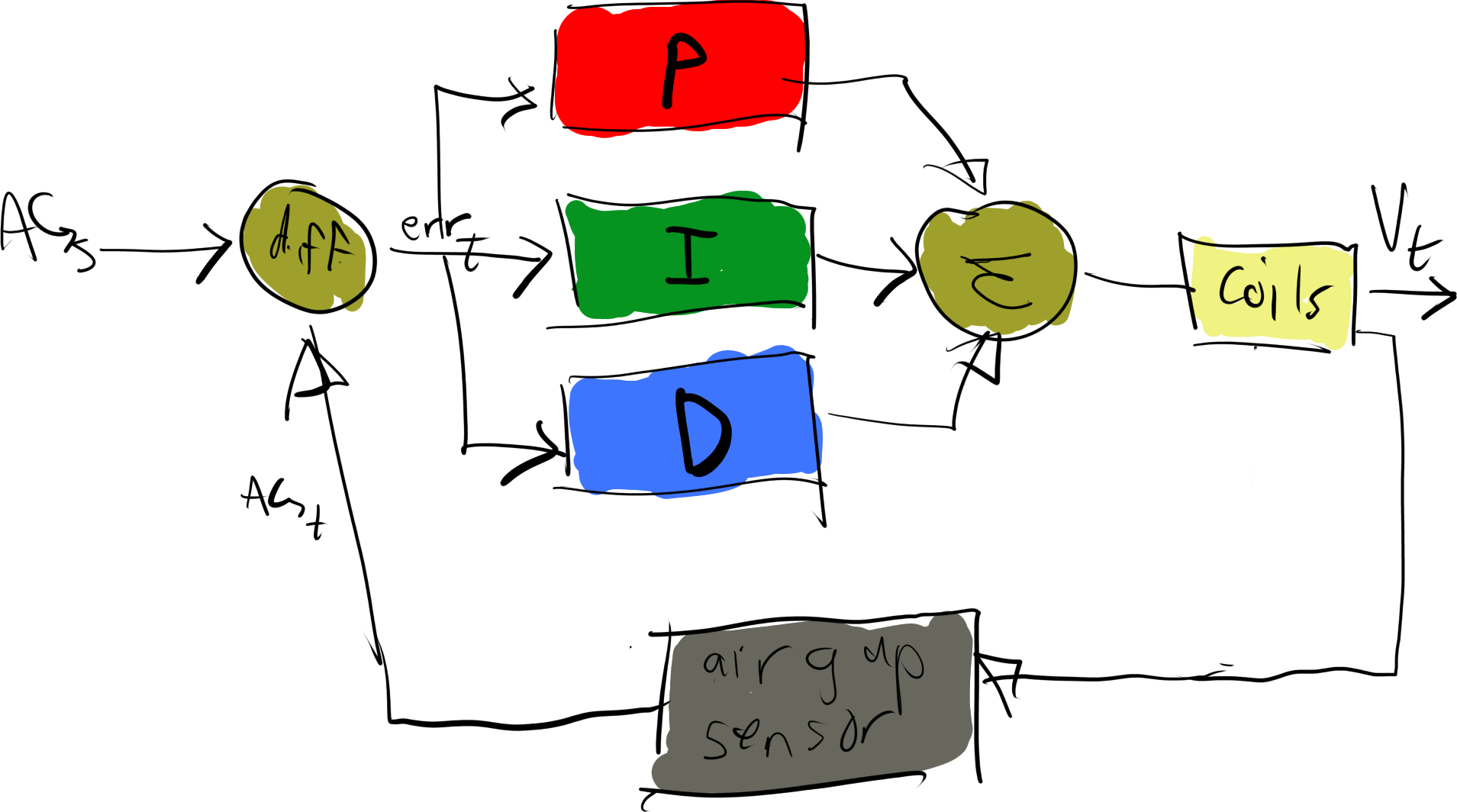
7. PID Controller

Now we get to our final objective: The PID controller. Again I need to scope limit here. Normally the PID controller will need some form of optimization of PID gain parameters K_p, K_i and K_d. Since this would essentially require the implementation of PID autotuner, which requires some time, I’ve not implemented it. Instead, I’ve opted for the trial and error approach to setting these parameters for the sake of demonstration. The parameters I’ve arrived at are the following: K_P = 5, K_i= 0.2 and K_D = 0.05. These are non-optimal – these need fiddling to produce a desirable graph that shows the dynamics of the system in an interesting way for a specific air gap. I’ve chosen an air gap of 7 mm. In practice, after auto-tuning with the real system they should capture the real response characteristics of both the resonant circuit of the coil track assembly but also the inertial characteristics.

My modeling of the PID system will follow the same approach as that of traditional PID systems as shown in figure 8 below. In this system, we would start the simulation at time zero with the coil assembly (primary) sitting on the track (secondary). After this the system will measure the air gap as zero and start by computing the error between our set point of AG_s = 7 mm. The error will be multiplied (P), integrated (I) and differentiated (D) using time discretized calculus. Once complete the summed P, I and D terms should, if tuned properly output a voltage value

We can code this in python as follows in the code below. Notice here that the try and catch block in the code is for situation where a scalar or vector input is provided.

With this function: pid_airgap_calculation (ag0, err0, agS, vmax, int0, kp, ki, kd) written. We can now update our PID controller loop from section 6 as shown in the code below:

Notice that in the second half of the code after the pid_airgap_calculation() function, I have some additional coding steps. The first of these voltages aimed at estimating the PWM output voltage waveform of the microcontroller via the code shown below. See section 3 on voltage sources for further details.

The second code snippet is shown below. This is designed to go through each phase of the PWM output waveform and apply smoothing. This would essentially emulate somewhat the low pass filter that might be connected to the output of the MCU to recreate a sinusoidal waveform as seen by the coils. It might also include the coils and their inductance related impacts. Note that this is another one of those time average approaches. Is it correct? No. But it does the job for a quick and dirty approach.

Once a PID output voltage is computed, we need to update our simulation model. Here I use magpylib to set the coil current based on the PWM output.

Of-course, I need not do that, I could also use the triangle wave directly or the average output voltage to do this same thing as shown below. Below, I’ve used the output voltage as computed directly by the pid_airgap_calculation() function.

With this all said and done, there is one last snippet of code that aims to update the model output. This next code below, basically assigns the average equilibrium air gap of all three coils to the model and thus changes the display to show that the coil real air gap position after all calculations are done – this is the air gap at the last time step of the simulation.

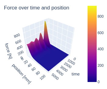
From this PID control we can actually graph a few details as well. For instance. We can plot the forces generated by the track on the coil as the PID controller functions as shown in figure 9.

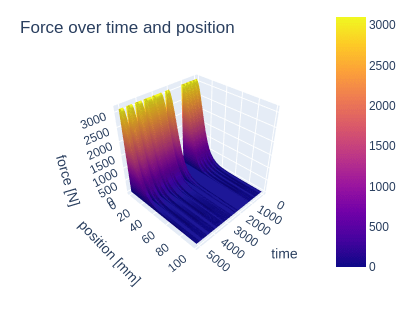
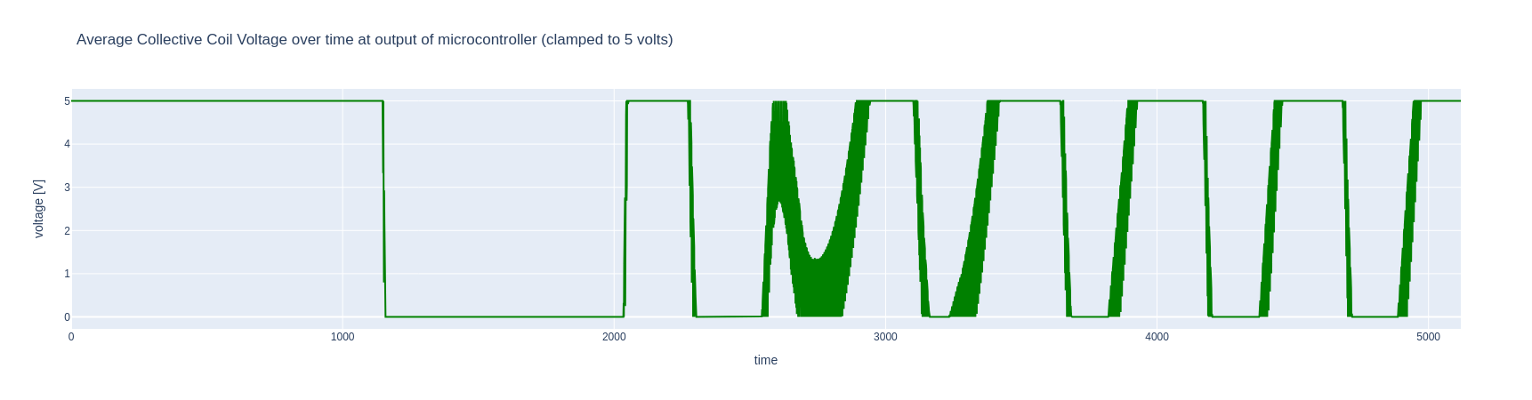
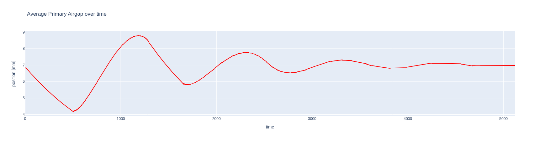
In addition we can also start to look at the output of the PID controller in terms of the position of the coils assembly relative to the track. See figure 10. Here we see that there is some oscillation of the air gap resulting from the on and off switching of the PWM signal. As time passes by the coil position approaches the air gap desired (i.e. AG_s = 7 mm). However, the combined impacts of the oscillation of the PWM signal and the poor damping as a result of guess work associated with the PID gain parameters, leads to an inability to reach a completely steady state air gap.

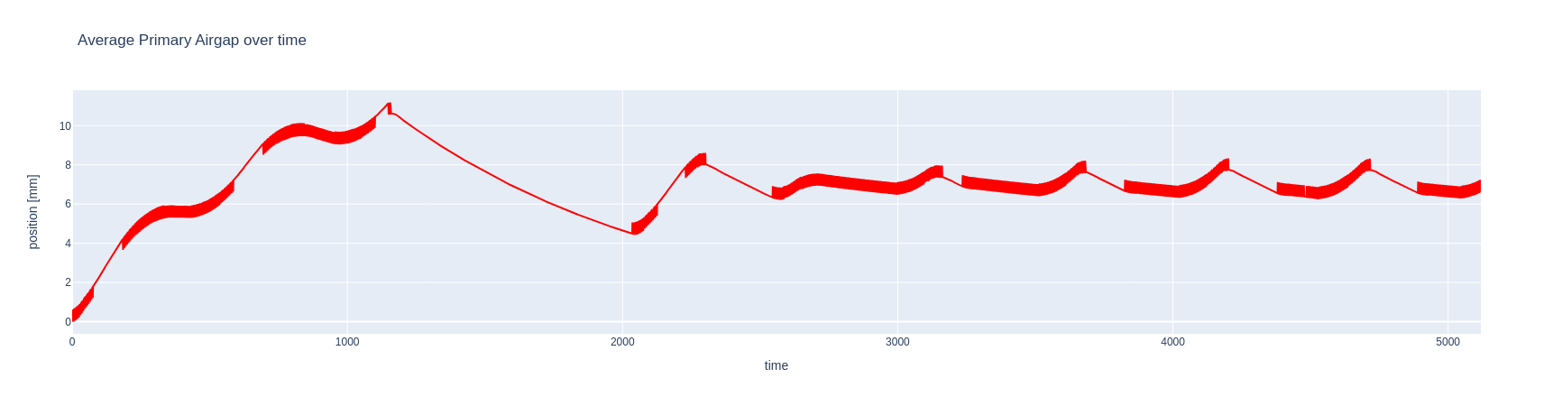
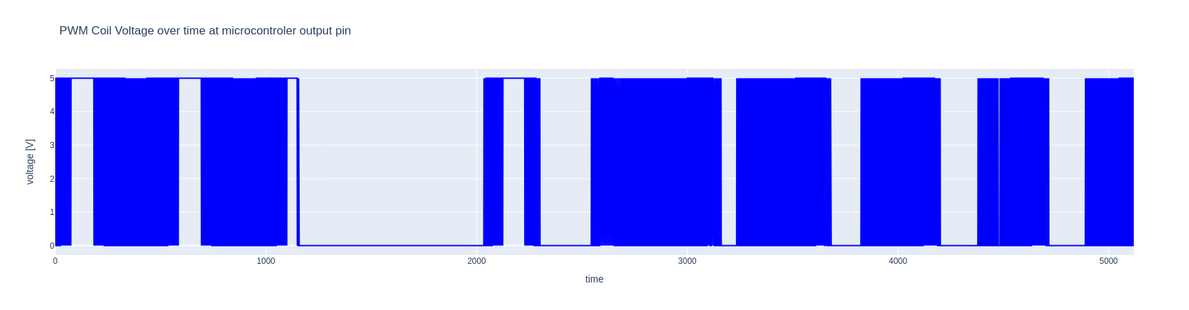
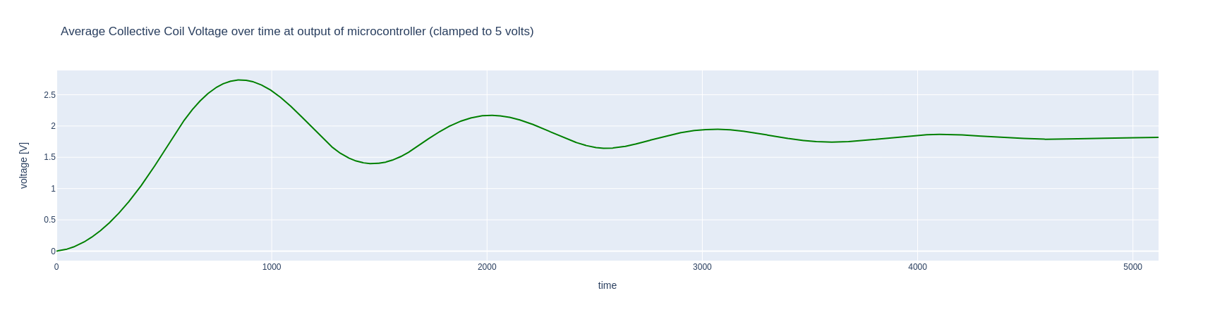
Following along we can also look at the voltage waveform and the PWM waveform leading to this air gap positioning as shown in figure 10 and figure 11. Notice that in the case of figure 10, the voltage waveform is clipped to the limits of the output of the microcontroller.

We can also verify that the air gap distance in figure 9 resulting from the PID control can also be seen more clearly following text book examples as follows in figure 12 and figure 13. Note that I’ve made some adjustments to the PID gain parameters as follows for this case: K_P = 0.01; K_I = 0.002; K_D = 0.001. Notice that the air gap graph in figure 12 isn’t smooth like that of figure 13. This is likely because the nearest neighbour approach to force estimation leaves the air gap estimation somewhat disjointed.

From this non-pwm version of the PID controller, we see that we can produce a force plot that shows the oscillation behaviour resulting from the over and under correction of the controller as in figure 14.

8. Conclusion

So with that we can conclude by saying that I’ve shown you a quick and dirty approach to simulating the PID control of the air gap of a Linear Induction Machine. Here in this machine, the vertical position of levitating a primary set of coils is computed and controlled. I’ve emulated the use of an air gap sensor by using magpylib to compute the B-field -> Force field -> Equilibrium Air Gap at every time step of the simulation and then generating the next time step voltage of the coils for control of this equlibrium air gap.

The resulting full code for this simulation attempt can be found by clicking the link below. Included is a Jupyter Notebook. Happy coding and good luck.

References

1. Micheal Ortner, Lucas GabrielColiado Bandeira. Magpylib: A free Python package for magnetic field computation. Published 2020. https://doi.org/10.1016/j.softx.2020.100466
2. The Magpylib Documentation. Last Accessed: September 2023. https://magpylib.readthedocs.io/en/latest/index.html